New Perspectives Excel 365/2021 | Module 10: SAM Project 1a Lighting Designs

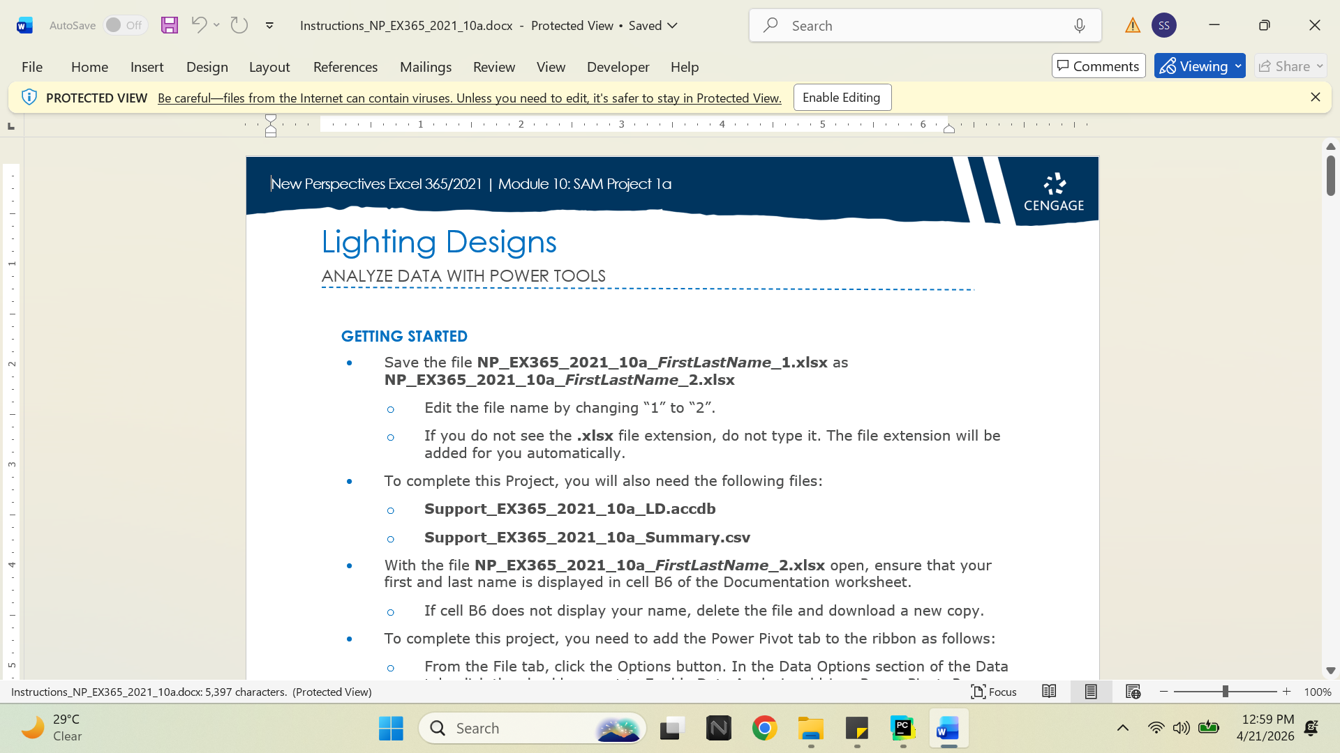
GETTING STARTED

1. Save the file NP_EX365_2021_10a_FirstLastName_1.xlsx as NP_EX365_2021_10a_FirstLastName_2.xlsx

a. Edit the file name by changing “1” to “2”.

b. If you do not see the .xlsx file extension, do not type it. The file extension will be added for you automatically.

2. To complete this Project, you will also need the following files:

Support_EX365_2021_10a_LD.accdb

Support_EX365_2021_10a_Summary.csv

3. With the file NP_EX365_2021_10a_FirstLastName_2.xlsx open, ensure that your first and last name is displayed in cell B6 of the Documentation worksheet.

a. If cell B6 does not display your name, delete the file and download a new copy.

4. To complete this project, you need to add the Power Pivot tab to the ribbon as follows:

a. From the File tab, click the Options button. In the Data Options section of the Data tab, click the checkbox next to Enable Data Analysis add-ins: Power Pivot, Power View and 3D Map, and click OK.

PROJECT STEPS

1. Jacob Sherman is the director of sales for Lighting Designs, a store and website that caters to building contractors in five locations in the Seattle area. Jacob asks for your help in producing a sales report. He wants to analyze sales for the past year and project future sales for all the stores. To create the report, you need to import data from various sources and use the Excel Power tools. Go to the Sales Summary worksheet, where Jacob wants to display a summary of the company's annual sales since the first store opened in the year 2003. He has a text file that already contains this data. Use Power Query to create a query and load data from a CSV file into a new table as follows:

a. Create a new query that imports data from the Support_EX365_2021_10a_Summary.csv text file.

b. Edit the query to remove the Units Sold and Notes columns.

c. Close and load the query data to a table in cell A2 of the existing worksheet.

2. Go to the Previous Year worksheet, which lists the sales per month for the previous year in a table and compares the sales in a chart. Jacob imported this data from the Orders table in an Access database. He wants to track the changes in monthly sales and project the first six months of this year's monthly sales. Create a forecast sheet as follows to provide the data Jacob requests:

a. Based on the data in the range A2:B14, create a forecast sheet.

b. Use 6/30/2025 as the Forecast End date to forecast the next six months.

c. Use Six Month Forecast as the name of the new sheet.

d. Resize and move the forecast chart so that the upper-left corner is within cell C2 and the lower-right corner is within cell E12.

3. Go to the Stores worksheet. Jacob wants to display information about lighting products purchased according to store and manufacturer. He has been tracking this data in an Access database. Import the data from the Access database as follows:

a. Create a new query that imports data from the Support_EX365_2021_10a_LD.accdb database.

b. Select the 2024_Orders, Products, and Purchases tables for the import.

c. Only create a connection to the data and add the data to the Data Model. On the Stores worksheet, Jacob wants to show the categories of products sold in each of the company's five stores during 2024.

d. In cell A2 of the Stores worksheet, use Power Pivot to insert a PivotTable based on the data in the 2024_Orders table.

4. Edit the PivotTable as follows to provide this information for Jacob:

a. Use the following fields from the 2024_Orders table in the PivotTable: · Category field for the row headings · StoreCity field for the column headings · ItemQty field for the values

b. Use Products Sold as the custom name of the Sum of ItemQty field.

c. In cell A3, use Lighting Products to replace "Row Labels", and then resize column A to its best fit.

d. In cell B2, use Stores to replace "Column Labels".

5. Jacob occasionally would like to focus on the number of lighting products sold in the five stores per month. Add a Timeline Slicer as follows to the Stores worksheet:

a. Insert a Timeline Slicer that uses the OrderDate field from the 2024_Orders table.

b. Move and resize the Timeline Slicer so it covers the range A12:G18.

c. Scroll the Timeline Slicer to display all periods.

6. Jacob also wants to examine the percentage each type of lighting product contributed to total sales in each store. Create a PivotChart as follows:

a. Based on the PivotTable on the Stores worksheet, create a 100% Stacked Column PivotChart.

b. Move and resize the PivotChart so that its upper-left corner is in cell H2 and its lower-right corner is in cell N16.

7. Go to the Manufacturers worksheet. Jacob wants to compare products sold by category and manufacturer. This data is stored in the Purchases and Products tables. Create a PivotTable as follows that provides the products sold by manufacturer information for Jacob:

a. In cell A2, use Power Pivot to insert a PivotTable in the Manufacturers worksheet.

b. Use the following fields in the PivotTable: · Manufacturer field from the Products table for the row headings · Category field from the Products table for the column headings · ItemQty field from the Purchases table for the values

8. In order to relate the data in the Products and Purchases tables to make a proper comparison, use the Power Pivot window to create a relationship between the Purchases and Products tables based on the ItemID field.

9. Jacob asks for another way to visualize the products sold by manufacturer. Create a PivotChart as follows:

a. Based on the PivotTable on the Manufacturers worksheet, create a Stacked Bar PivotChart.

b. Move and resize the PivotChart so that its upper-left corner is within cell I2 and its lower-right corner is within cell O25.

c. Hide all the field buttons in the PivotChart.

10. Jacob also wants to be able to focus on a single category of product at a time. Add a slicer to the PivotChart as follows:

a. Add a slicer based on the Category field from the Products table.

b. Move the slicer below the PivotChart so that it covers the range I26:K38.

c. Use the slicer to filter the PivotTable and PivotChart to show only products in the Commercial category.

Your workbook should look like the Final Figures on the following pages. Save your changes, close the workbook, and then exit Excel. Follow the directions on the website to submit your completed project.

Final Figure 1: Sales Summary Worksheet

Final Figure 2: Six Month Forecast Worksheet

Final Figure 3: Previous Year Worksheet

Final Figure 4: Stores Worksheet

Final Figure 5: Manufacturers Worksheet